Unlock a world of possibilities! Login now and discover the exclusive benefits awaiting you.
- Qlik Community
- :
- Forums
- :
- Analytics & AI
- :
- Products & Topics
- :
- App Development
- :
- Re: How to identify last 3 values in qliksense piv...
- Subscribe to RSS Feed
- Mark Topic as New
- Mark Topic as Read
- Float this Topic for Current User
- Bookmark
- Subscribe
- Mute
- Printer Friendly Page
- Mark as New
- Bookmark
- Subscribe
- Mute
- Subscribe to RSS Feed
- Permalink
- Report Inappropriate Content
How to identify last 3 values in qliksense pivot table and color it
Hello,
I am using total 4 fields. One field is for Pivot Dimension and 2 Fields as Columns and 1 field as Measure ( Sum(Sales)).
If I expand one of the column, I will get 7 values as sum(sales) . Is there any way to identify last 3 values and assign color for last 3 values. Can Someone please advise.
-Karthick.
- « Previous Replies
-
- 1
- 2
- Next Replies »
Accepted Solutions
- Mark as New
- Bookmark
- Subscribe
- Mute
- Subscribe to RSS Feed
- Permalink
- Report Inappropriate Content
Hi
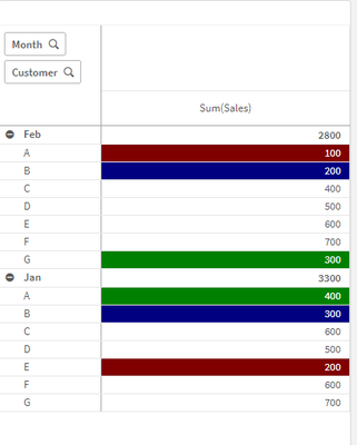
You can add a color condition based on Secondary Dimensionality like below. But if your users start moving dimensions and change format of the pivot I can't promise it will work
pick(SecondaryDimensionality(),white(),
pick(hrank(-sum(Sales),0,1),red(),blue(),green()))
- Mark as New
- Bookmark
- Subscribe
- Mute
- Subscribe to RSS Feed
- Permalink
- Report Inappropriate Content
Hi,
you can specify colors based on certain condition what is your condition for coloring ?
Vikas
If the issue is solved please mark the answer with Accept as Solution & like it.
If you want to go quickly, go alone. If you want to go far, go together.
- Mark as New
- Bookmark
- Subscribe
- Mute
- Subscribe to RSS Feed
- Permalink
- Report Inappropriate Content
Condition is , I am using measure as Sum(Sales). Each column has 7 records. So out of that 7 records, I need to find only the last 3 values in each column. like 7th last is green() , 6th last is blue(), 5th last is grey()
- Mark as New
- Bookmark
- Subscribe
- Mute
- Subscribe to RSS Feed
- Permalink
- Report Inappropriate Content
HI
Try something like below
Pick(Match(RowNo(),5,6,7)+1, black(), LightGray(), blue(), Green())
Please close the thread by marking correct answer & give likes if you like the post.
- Mark as New
- Bookmark
- Subscribe
- Mute
- Subscribe to RSS Feed
- Permalink
- Report Inappropriate Content
Thanks @MayilVahanan , But in your Example, for Feb Month , lowest 3 Sum(sales) is 100(A),200(B) and 230(H) . We need to give colors for those values only. 100 , 200 and 230
Also instead of row(in your example) , I am using column in my end. Do we have option for that?
-Karthick.
- Mark as New
- Bookmark
- Subscribe
- Mute
- Subscribe to RSS Feed
- Permalink
- Report Inappropriate Content
Any possible ways to achieve this please?
- Mark as New
- Bookmark
- Subscribe
- Mute
- Subscribe to RSS Feed
- Permalink
- Report Inappropriate Content
Hello
Use this to set your Background or Text Color:
pick(rank(-sum(Sales)),red(),blue(),green())
- Mark as New
- Bookmark
- Subscribe
- Mute
- Subscribe to RSS Feed
- Permalink
- Report Inappropriate Content
Hi @jbhappysocks ,
I have used the same formula, but its not working . I am looking the result in row wise.
For Ex: In first Row : 200000 ( min value ) - blue , 305368(2nd Min value) - green , 310000 ( 3rd min) - red().
All other fields should remain white.
- Mark as New
- Bookmark
- Subscribe
- Mute
- Subscribe to RSS Feed
- Permalink
- Report Inappropriate Content
If you want the rank by row in a pivot you use Hrank instead of Rank
pick(hrank(-sum(Sales),0,1),red(),blue(),green())
Example above is not showing a blue cell since A and D are both ranked as 1 -> B is ranked as 3.
- Mark as New
- Bookmark
- Subscribe
- Mute
- Subscribe to RSS Feed
- Permalink
- Report Inappropriate Content
Thanks @jbhappysocks . One last question.Its perfectly working if I expand each columns like 1, 2, 3, 4. Inside each column i have checked , last 3 values color is fine. But Is there any way to show normal white background , if the columns are not expanded.
Below screenshot , I have not expanded each column. but our background rule applied here as well. Do we have option to restrict that?
- « Previous Replies
-
- 1
- 2
- Next Replies »


