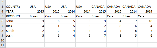
have you ever tried to load a spreadsheet that looks like this ?
Firstly , i believe that this spreadsheet is pretty straight forward spreadsheet, however this is not a trivial spreadsheet for Qlik to load because its formatted as pivot table with multiple (3) nested column headers.
How to load ?
If you were thinking crosstable then you are on the right track . This technique is articulated in an excellent video resource by Mike tarallo
But you'll need more if you want to unpivot each column into a tabular format that is ideal for Qlik:
The technique described here is to perform successive crosstable loads on the spreadsheet where each load reads just a single row (per column header) .
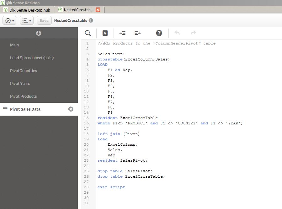
The Data Load Script:
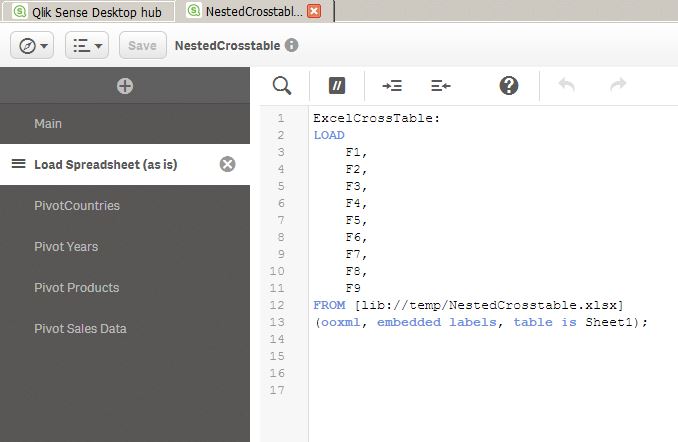
1. The first step is to load the spreadsheet without any transformation. I recommend doing this so that Qlik only reads the spreadsheet once which , if the spreadsheet is very large and complex, will make things quicker. The spreadsheet used here has no column names, so generic columns names "F1,F2,F3.." show up.
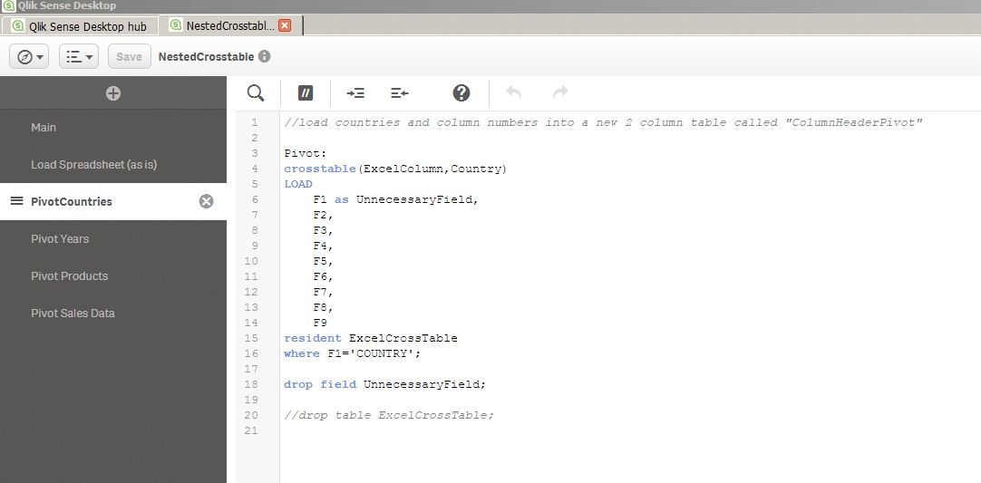
2. Next, we focus on loading the column identifiers (F1,F2 etc...) with the country values that appear in each column. The column identifier i have named 'ExcelColumn' . The first column does not actually have a country value in it , so i rename F1 to 'Unnecessaryfield' and drop it after the load. Also , this crosstable load is ONLY loading the 3rd row of the spreadsheet where F1='Country'.
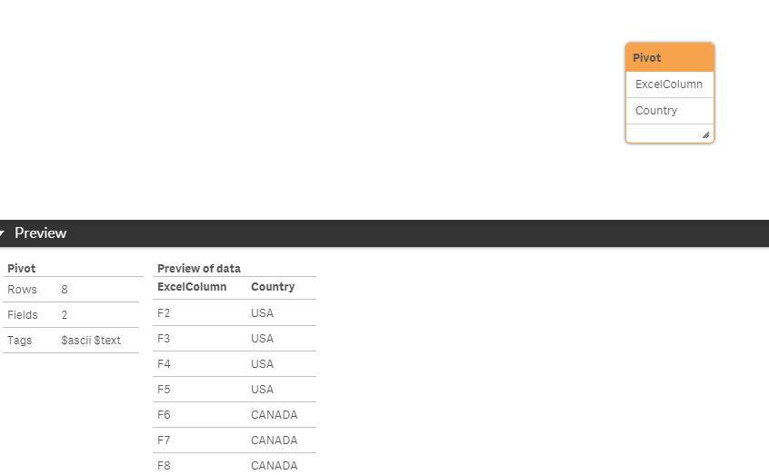
The result of this load is just a 2 column tabular data set that associates the ExcelColumn with a Country
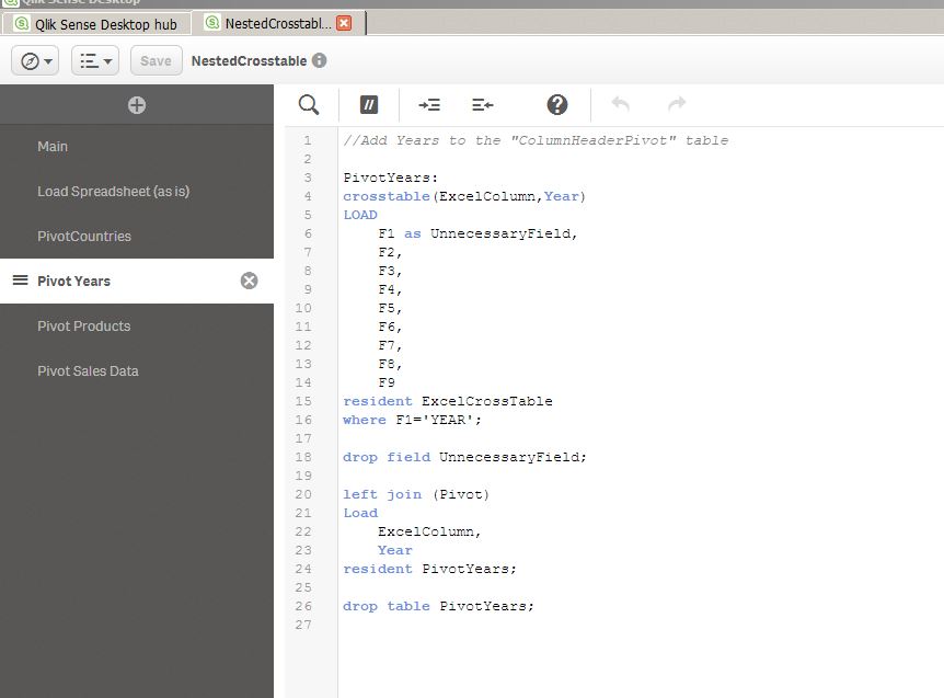
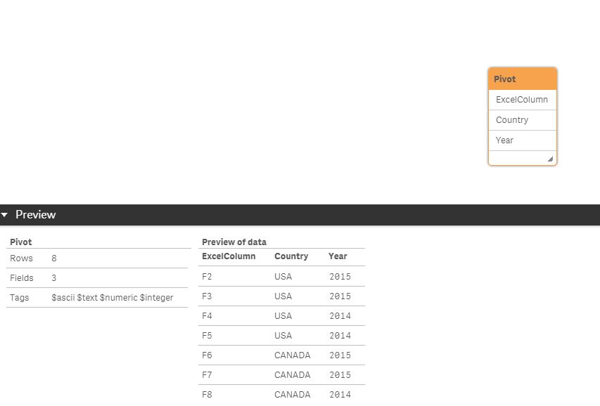
3. Next step is to use the same technique to load the YEAR row and then join the result to the 'Pivot' table above. As before, just a single row is read (F1='YEAR') , F1 is an unnecessary field with no product value that is dropped. Whats different is that i join the new 2 column table with ExcelColumn and YEAR to the existing 2 column table that has ExcelColumn and COUNTRY using a join statement.
This results in a 3 column table as below
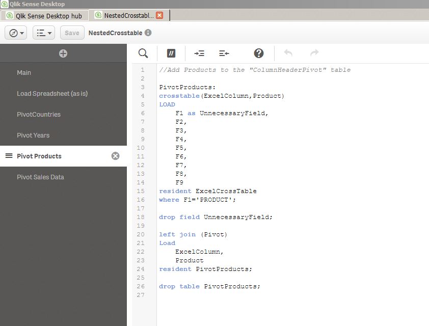
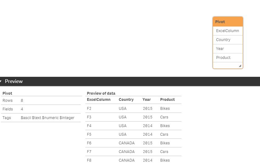
4. The technique repeats for the Products . Identical to step 3 except PRODUCT instead of YEAR
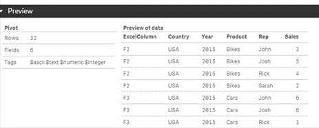
Now we have a 4 column table as below
5. Lastly we employ a proper crosstable load to load the row headers (Sales Reps) and all the actual sales numbers . The only rows not loaded are the PRODUCT,COUNTRY, and YEAR rows. Also, at the end the original spreadsheet table that was loaded is no longer needed