Unlock a world of possibilities! Login now and discover the exclusive benefits awaiting you.
- Qlik Community
- :
- All Forums
- :
- QlikView App Dev
- :
- Re: Background color headers pivot table
- Subscribe to RSS Feed
- Mark Topic as New
- Mark Topic as Read
- Float this Topic for Current User
- Bookmark
- Subscribe
- Mute
- Printer Friendly Page
- Mark as New
- Bookmark
- Subscribe
- Mute
- Subscribe to RSS Feed
- Permalink
- Report Inappropriate Content
Background color headers pivot table
Hello,
I added a pivot table to my sheet. Depending on the values shown in the columns, the background color of the headers should be changed.
Just as a start I used this formula to the Background Color setting of the dimension that goes with the headers:
=If ((Dimensionality() = 1) and (SecondaryDimensionality() <> 0), rgb(255,180,180))
I expected that all the headers, except the header for the total, would have a pinkish background.
To my surprise it was not so.
The headers for the columns of which the FIRST value was non existing were not colored.
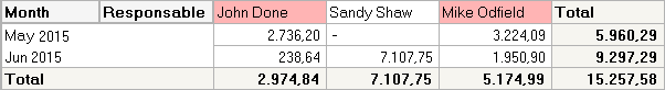
In the above example the header with name Sandy Show has no background color, because the first value (for May 2015) is not available.
Is this a bug in QlikView? How can this be solved?
RW
- Mark as New
- Bookmark
- Subscribe
- Mute
- Subscribe to RSS Feed
- Permalink
- Report Inappropriate Content
Hi, did You consider of use "Custom format cell"?
michał
- Mark as New
- Bookmark
- Subscribe
- Mute
- Subscribe to RSS Feed
- Permalink
- Report Inappropriate Content
Hi Rudy,
try like this:
1. Go to Dimension Tab--> Used Dimension ->Expand + symbol into used Dimensions->Background Color -> give your required Color
else
right click on the pivot table->format cell -> give color.
Thanks,
Divya
- Mark as New
- Bookmark
- Subscribe
- Mute
- Subscribe to RSS Feed
- Permalink
- Report Inappropriate Content
Thanks Michał,
but this is not applicable.
As I indicated in the intro of my question the background color of the headers should be changed depending on the values shown in the columns. Thus the color should be given by an expression.
A clearer description of the problem is given in the attached pdf document
RW
- Mark as New
- Bookmark
- Subscribe
- Mute
- Subscribe to RSS Feed
- Permalink
- Report Inappropriate Content
Thanks Divya,
but this is not applicable.
As I indicated in the intro of my question the background color of the headers should be changed depending on the values shown in the columns. Thus the color should be given by an expression.
A clearer description of the problem is given in the attached pdf document
RW
- Mark as New
- Bookmark
- Subscribe
- Mute
- Subscribe to RSS Feed
- Permalink
- Report Inappropriate Content
Hi, check this topic: Background color for pivot table cells with MISSING values