Pivot Table Dimension Condition Format

[Anonymous]

Hello,

I'm a beginner on QlikView, and I would modify my Pivot Table format with conditions on dimensions.

Here is the pivot table on QlikView:

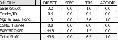
And the Excel:

Do you have an idea ? For example for the forecolor of the partial sum named "Total Staff" ?

Thank you in advance for your help,

Cocalero.

[Chanty4u]

can u explain more?

u want to modify the table format means?

if yes   in style  tab there is  current style   ----> drop down u can select there.

if not explain?

[Anonymous]

Do you want  to display Total as Total Staff ? if it is the case go to Presentation tab and give your desired name in the

Labels for Totals

[tamilarasu]

Hi,

You can use dimensionality() in your text expression like below.,

If(Dimensionality()=0,RGB(28,75,240))

[Chanty4u]

If u want to chnge the colurs based on dimensions or epxresions

as tamil said use dimenionality() or

u can use custom format cell  also.

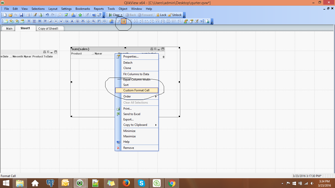
go to -->view---> design grid--->

select ur table --->right clik---> custom format cell----> select ur columns  or rows----->and select colur and apply.

[avinashelite]

if you want the Total to have different color than you could use the Dimensionality() function

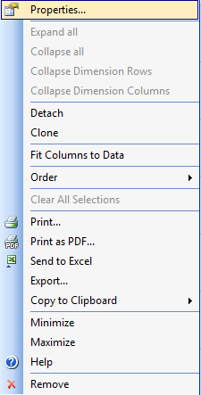
Go to > expression > you will see + mark >click on it you will the background color option > paste the expression

If(Dimensionality()=0,blue())

To change the Label header color then > click on design grid from the design tool bar > right click on the label header > custom format cell > and the color you want

[Digvijay_Singh]

Just right click on table and use Custom cell option.

[#8]

Give a right click on report and then---> custom format cell----> select your columns  or rows--->select your desired color and apply.

[Anonymous]

Sorry, but i don't see this option and my table. I have:

[Chanty4u · Accepted solution]

chk dis

or else go to view tab there u will find grid view option clik on that