Highlighting top n values in each column of a table

[linoyel]

Hey all!

I have a straight table with calculated expressions (presented in percents).

2 questions:

1. How to add min, max and average for each column?

2. How to highlight top 5 values in each column? (say if I have 5 columns, I need 25 values to be highlighted)

3. How to highlight today's day? (see in the below example that "22" is red)

Thank you!

Below is the example of how my table is supposed to look like:

Day / Billing Country	Saudi Arabia	United Arab Emirates	Turkey	United States	Egypt	France	South Africa	Russia	Singapore	Qatar	Kuwait	Malaysia	Nigeria	Brazil	Italy	Lebanon	United Kingdom	Venezuela
1	48%	47%	61%	68%	33%	44%	37%	28%	48%	35%	32%	32%	9%	27%	36%	36%	29%	55%
2	51%	39%	49%	69%	31%	48%	30%	31%	58%	39%	36%	32%	30%	49%	33%	30%	43%	52%
3	43%	46%	53%	56%	34%	51%	33%	30%	56%	41%	26%	43%	21%	49%	29%	33%	38%	47%
4	49%	44%	52%	59%	28%	51%	32%	28%	61%	42%	41%	42%	19%	50%	44%	16%	48%	55%
5	44%	42%	53%	56%	34%	61%	35%	27%	54%	34%	38%	37%	8%	48%	29%	33%	47%	55%
6	44%	46%	52%	63%	35%	49%	30%	30%	51%	39%	30%	31%	40%	56%	34%	45%	48%	51%
7	46%	40%	51%	59%	36%	55%	28%	29%	51%	44%	28%	25%	28%	63%	35%	31%	40%	55%
8	44%	37%	50%	70%	31%	53%	30%	36%	45%	36%	32%	32%	16%	43%	30%	30%	41%	59%
9	43%	40%	54%	66%	30%	59%	36%	31%	57%	42%	23%	39%	18%	40%	31%	25%	38%	50%
10	45%	44%	57%	61%	40%	53%	31%	28%	50%	30%	29%	29%	8%	41%	43%	29%	36%	45%
11	47%	44%	51%	60%	29%	59%	32%	33%	47%	43%	33%	44%	40%	31%	44%	24%	28%	63%
12	45%	41%	53%	68%	27%	63%	37%	29%	41%	40%	40%	43%	29%	65%	44%	31%	39%	44%
13	43%	37%	55%	52%	24%	58%	32%	33%	43%	28%	33%	27%	25%	54%	36%	34%	32%	43%
14	41%	38%	51%	65%	33%	48%	28%	30%	41%	48%	24%	36%	12%	33%	42%	32%	49%	55%
15	43%	45%	61%	65%	34%	44%	33%	28%	47%	48%	34%	39%	9%	52%	40%	27%	36%	58%
16	49%	46%	60%	61%	33%	57%	39%	34%	47%	26%	34%	30%	39%	41%	43%	31%	44%	55%
17	54%	46%	55%	65%	38%	48%	28%	32%	47%	32%	32%	33%	27%	59%	25%	34%	46%	42%
18	46%	40%	56%	69%	24%	51%	30%	28%	44%	33%	22%	35%	25%	58%	33%	35%	10%	49%
19	46%	38%	57%	62%	27%	48%	24%	35%	49%	37%	32%	39%	46%	55%	20%	31%	48%	57%
20	44%	38%	52%	64%	27%	45%	36%	29%	38%	43%	33%	25%	27%	50%	20%	19%	26%	53%
21	43%	38%	45%	55%	30%	53%	28%	34%	33%	39%	25%	17%	5%	28%	49%	29%	28%	54%
22	45%	42%	52%	64%	31%	39%	32%	30%	41%	31%	28%	40%	23%	40%	33%	30%	25%	49%
23	40%	33%	56%	65%	38%	38%	31%	32%	34%	31%	45%	40%	33%	35%	22%	29%	32%	55%
24	43%	40%	51%	64%	34%	49%	37%	30%	40%	32%	34%	42%	0%	43%	34%	32%	39%	48%
25	45%	35%	54%	61%	30%	45%	30%	31%	45%	31%	27%	35%	20%	42%	37%	28%	61%	47%
26	49%	38%	49%	67%	27%	47%	29%	36%	41%	40%	19%	22%	17%	50%	21%	24%	42%	55%
27	43%	40%	53%	71%	34%	44%	34%	33%	28%	32%	19%	32%	18%	53%	35%	34%	51%	43%
28	42%	39%	47%	69%	36%	45%	38%	35%	35%	36%	36%	33%	16%	38%	33%	33%	39%	50%
29	46%	47%	52%	59%	34%	48%	33%	33%	55%	36%	33%	25%	16%	27%	40%	36%	28%	49%
30	41%	42%	47%	63%	41%	50%	34%	31%	45%	52%	43%	26%	29%	45%	41%	25%	34%	51%
31	41%	41%	50%	65%	34%	50%	29%	25%	56%	42%	36%	47%	29%	82%	32%	42%	67%	44%
min	40%	33%	45%	52%	24%	38%	24%	25%	28%	26%	19%	17%	0%	27%	20%	16%	10%	42%
max	54%	47%	61%	71%	41%	63%	39%	36%	61%	52%	45%	47%	46%	82%	49%	45%	67%	63%
avg	45%	41%	53%	63%	32%	50%	32%	31%	46%	38%	32%	34%	22%	47%	35%	31%	39%	51%

[#2]

Can u attach ur sample application??

[its_anandrjs]

You have to use this conditions in the expressions background where you have to give conditions for coloring of the cell based on the condition and calculate MAX, MIN , AVG and Today() date and display in the chart. If you have any sample then provide might be easy.

[linoyel]

Hi Anand,

What do you mean by providing a sample?

I've attached the whole table from my Qlikview, it's just that I first transferred it to excel in order to highlight what I need and make min, max and average calculations...

[tresesco]

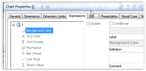
You have to write expression for background color:

And yes, for sharing qvw look: Preparing examples for Upload - Reduction and D... | Qlik Community

[its_anandrjs]

I mean raw data

3 for date write in background color If([Day / Billing Country] = Day(today()),Red())

[its_anandrjs]

For third option write like in background option

=if(Max(Saudi Arabia) > 5 ,Green())   // write this code for all expression and change the expression

Ex:-

1st Expresssion

=if(Max(Saudi Arabia expression) > 5 ,Green())

2nd Expression

=if(Max(United Arab Emirates expression) > 5 ,Green())

[bertdijks]

I copied the data you provided in attached excel and used it in the solution.

As suggested I used the format in the dimension-expression attrributes

For the last 3 rows I used 3 seperate extra loads. To Ensure the right order in the table, I converted the day field to a dual type, sorted on numeric value and show tekst.

I hope this helps!

Bert

[Gysbert_Wassenaar]

See attached example.

[its_anandrjs]

Hi Linoy,

On the basis of your attached data i provide you the load script of the application and how to design the pivot table in the front end i give information about that to you.

//Load your table like below script

CrossTable([Billing Country], Data)

LOAD [Day / Billing Country],

     [Saudi Arabia],

     [United Arab Emirates],

     Turkey,

     [United States],

     Egypt,

     France,

     [South Africa],

     Russia,

     Singapore,

     Qatar,

     Kuwait,

     Malaysia,

     Nigeria,

     Brazil,

     Italy,

     Lebanon,

     [United Kingdom],

     Venezuela

FROM

RawData.xlsx

(ooxml, embedded labels, table is Sheet1);

Then take a Pivot table

Dimension1:- [Day / Billing Country]

Dimension2:- [Billing Country]

Expression:- Sum(Data)

Then for points that you ask is

1. for this you have to add another pivot table and add

Diemnsion:-  [Billing Country]

Expressions

for Min =Min(Data)

for Max =Max(Data)

for Avg =Avg(Data)

2.  Click on the + on Sum(Data)

for Background :- if(rank(sum(Data)) <= 5 ,RGB(183,255,255))

for Text Color :- if(rank(sum(Data)) <= 5 ,Black())

for Tex Format :- if(rank(sum(Data)) <= 5 ,'<B>')

3. Click on the + on [Day / Billing Country] and type

for Background :- =if([Day / Billing Country] = Day(Today()),RGB(255,157,157))

for Text Color :- =if([Day / Billing Country] = Day(Today()),Black())

for Text Format :- =if([Day / Billing Country] = Day(Today()),'<B>')

Regards